
Thermal Conductivity

The Most Accurate and Reliable Equipment with Superior Reproducibility – Unmatched in Korea!
OVERVIEW
This device measures the thermal conductivity of various materials using the thermal equilibrium drop method according to the ASTM D5470 standard from the United States. It employs copper pillars for upper cooling and lower heating, determining the thermal conductivity of the specimen when thermal equilibrium is achieved. The total heat flow Q under steady-state conditions can be calculated using the following formula, where λ is the thermal conductivity of copper, A is the cross-sectional area of the copper, dA is the distance between the copper pillars, and ΔT is the temperature difference between the thermocouples attached to the copper pillars:

After raising the temperature to a specific level and reaching thermal equilibrium, the temperatures at the top and bottom of the copper pillars are measured simultaneously. The thermal conductivity is then calculated using the provided formula. The basic theory involves conducting two measurements with specimens of the same material but different thicknesses to eliminate the effects of contact resistance between the specimen and the pillars. By taking the reciprocal of the difference in thermal resistance and multiplying it by the thickness difference of the specimens, the thermal conductivity is determined.
If preparing samples of the same material with different thicknesses is not feasible, a single measurement can still be used to estimate the thermal conductivity. However, this method inherently includes some error due to the inability to account for contact resistance between the specimen and the copper pillars.
TECHNICAL SPESIFICATION
| Category | Vertical | Horizontal | Tolerance |
|---|---|---|---|
| ASTM Standard | ASTM D 5470 | Angstrom’s Method | |
| Standard Square Specimen Size | 22mm | ±0.2mm | |
| Standard Circular Specimen Size | 25mm | ±0.2mm | |
| Minimum Applicable Thickness | 0.02mm | ||
| Maximum Allowable Thickness | 10mm | ||
| Flatness (Non-elastic Specimens) | ±0.01mm | ||
| Measurement Range | 0.1–80 W/m·K | 0.1–1,000 W/m·K | |
| Thermal Resistance Range | 0.05–5.0 °C/W | Thermal Diffusivity Min. 0.02 m²/sec | |
| Pillar Pressure Range | 10–500 psi | 10–500 psi | |
| Pillar Pressure Accuracy | ±0.01% (at full span) | ±0.01% (at full span) | |
| Operating Temperature Range | 40–100 °C | 25–70 °C | |
| Features | ±0.001 °C resolution | ||
| Applications & Samples | Thermal tapes, Heat sinks, Ceramics, Metal foils, Insulating materials, Metals | ||
| Equipment Weight | 30kg | ||
| Equipment Dimensions | 360(L) × 310(W) × 630(H) mm | ||
| Power Supply | 220V AC, 60Hz, 100W |
TECHNICAL DETAIL
-
Complete Double Blocking of External Heat Transfer Factors: The device features an environment cover to fully isolate external temperature influences that could affect measurements.
-
Automatic Distance Adjustment and Pressure Display for ASTM D5470 Sample Types (1, 2, 3): The system automatically adjusts the distance between samples according to ASTM D5470 standards and displays the applied pressure for verification.
-
One-Click Positioning & Measurement with Auto-Position Memory: The device allows quick and precise sample positioning with a single click, thanks to its automated position memory function.
-
Advanced Program for Automatic Cooling Control per ASTM D5470: An innovative cooling control program ensures compliance with ASTM D5470 requirements for accurate thermal testing.
-
High-Precision RTD Sensors for Accurate Temperature Readings: The system uses high-accuracy Resistance Temperature Detectors (RTDs) to ensure reliable and precise temperature measurements.
This device measures the thermal conductivity of various materials using the ASTM D5470 standard (thermal equilibrium method). It employs copper pillars for top cooling and bottom heating, determining the thermal conductivity of the specimen when steady-state heat flow is achieved.
Key Equations & Principles
-
Heat Flow Calculation
The total heat flow (Q) under steady-state conditions is given by:Where:
-
= Thermal conductivity of copper
-
= Cross-sectional area of the copper pillar
-
= Distance between copper pillars
-
= Temperature difference between thermocouples (T.C) on the pillars
-
-
Thermal Conductivity Determination
-
After stabilizing at a target temperature, the device measures the top and bottom temperatures of the copper pillars.
-
Thermal conductivity is calculated using the above formula.
-
Two-Thickness Method (Recommended for Highest Accuracy)
-
Two measurements are taken using same-material specimens of different thicknesses.
-
This eliminates contact resistance errors between the specimen and copper pillars.
-
The thermal conductivity (λ) is derived by:
-
Taking the inverse of the thermal resistance difference,
-
Multiplying by the thickness difference of the specimens.
-
Single Measurement (Alternative with Potential Error)
-
If preparing two thicknesses is impossible, a single measurement can estimate thermal conductivity.
-
However, this method cannot eliminate contact resistance, leading to some theoretical error.

Basic Theory (Horizontal Type) – Thermal Conductivity Measurement System
This device employs Angström’s Method to determine thermal conductivity by:
-
Measuring temperatures at two fixed points along a sample from a heat source.
-
Calculating thermal diffusivity (α), then combining it with the material’s density (ρ) and specific heat (c) to derive thermal conductivity (λ).
Key Equations & Principles
1. Thermal Diffusivity (α) Calculation
Angström’s Method derives thermal diffusivity using:

Where:
-
= Harmonic number
-
= Driving frequency (ω=2πP)
-
= Distance between thermocouples
-
= Phase difference (ϕ=2πΔtPe)
-
= Temperatures at near/far points from the heat source
-
= Thermal wave period
-
= Effective period (Pe=Pn)
2. Simplified Practical Formula
For low driving frequencies (experimental conditions), thermal diffusivity reduces to:

3. Final Thermal Conductivity (λ)
Multiply thermal diffusivity (α) by density (ρ) and specific heat (c):